Tutorial

$$\newcommand{\vt}[1]{\boldsymbol{#1}} \newcommand{\uv}[1]{\hat{\boldsymbol{#1}}} \newcommand{\arr}[1]{\mathsf{#1}} \newcommand{\mat}[1]{\boldsymbol{\mathsf{#1}}}$$

In this tutorial we will go through the steps required for the formulation and the solution of the scattering of a time harmonic electromagnetic wave by a rectangular plate by means of the solution of the electric field integral equation.

Building the geometry

The sibling package CompScienceMeshes provides data structures and algorithms for working with simplical meshes in computational science. We will use it to create the geometry:

using CompScienceMeshes, BEAST
o, x, y, z = euclidianbasis(3)

h = 0.2
Γ = meshrectangle(1.0, 1.0, h)
@show numvertices(Γ)
@show numcells(Γ)

numvertices(Γ) = 36
numcells(Γ) = 50

Next, we create the finite element space of Raviart-Thomas aka Rao-Wilton-Glisson functions subordinate to the triangulation Γ constructed above:

X = raviartthomas(Γ)

The scattering problem is defined by specifying the single layer operator and the functional acting as excitation. Here, the plate is illuminated by a plane wave. The actual excitation is the tangential trace of this electric field. This trace be constructed easily by using the symbolic normal vector field n defined as part of the BEAST package.

κ = 1.0
E = Maxwell3D.planewave(direction=ẑ, polarization=x̂, wavenumber=κ)
e = (n × E) × n

The single layer potential is also predefined by the BEAST package:

t = Maxwell3D.singlelayer(wavenumber=κ)

It corresponds to the bilinear form

$$t(\vt{k},\vt{j}) = \frac{1}{ik} \int_{\Gamma} \int_{\Gamma'} \nabla \cdot \vt{k}(x) \nabla \cdot \vt{j}(y) \frac{e^{-ik|x-y|}}{4\pi|x-y|} dy dx - ik \int_{\Gamma} \int_{\Gamma'} \vt{k}(x) \cdot \vt{j}(y) \frac{e^{-ik|x-y|}}{4\pi|x-y|} dy dx$$

Using the LinearForms package, which implements a simple form compiler for Julia (@varform), the EFIE can be defined and discretised by

@hilbertspace j
@hilbertspace k
efie = @discretise t[k,j]==e[k]  j∈X k∈X

Solving and computing the values of the induced current in the centers of the triangles of the mesh is now straightforward:

u = solve(efie)
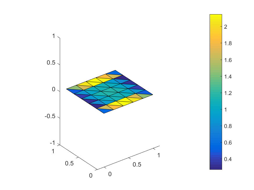
fcr, geo = facecurrents(u,X)

The resulting current distribution can be visualised by e.g. Matlab, Paraview, Plotly,...